Scholarship hypothetically makes men wiser, many times though it
gets one stubborn…. Don’t get perplexed! With all the intricacy involved, the
rudiments are straightforward.
The concept of PPS
originated with the man’s quest in space. The atomic clocks orbiting around the
earth in GPS satellites are utilized to obtain accurate timing. Today PPS is found in applications requiring
synchronization such as cellular networks, telecommunications timing, digital
TV and radio transmission, calibration laboratory systems, internet, stock market, computer games and precision stuff
like surveys where various data have to correspond in respect to time.
The
atomic clocks in the GPS satellites are monitored and compared to 'master
clocks' by the GPS Operational Control Segment; this 'GPS time' is steered to
within one microsecond of Universal Time. GPS receivers provide 1PPS output
signal. This pulse normally has a rising edge aligned with the GPS second, and
is used to discipline local clocks to maintain synchronization with Universal
Time (UT).
Time is crucial in
hydrographic multi beam survey because each piece of data received from a
device is immediately stored in the raw data files, in order to correlate it
with data coming from other devices, i.e. motion sensors, heading, position and
sound velocity, we need to stamp the time the measurement was taken.
This note is in particular relevance with offshore
hydrographic survey….but in general, it will be good in all relevant contexts.
While
totally rigorous testing of timing pulses requires an atomic clock reference,
useful information can be gathered using a survey-grade, dual-frequency GPS
receiver as the timing reference.
There
is a time difference (offset) in different GPS receivers. The standard
deviation of this offset provides a measure of the pulse stability or 'jitter'.
There are two factors to be considered in judging performance, one is the
average offset time and the other is the standard deviation of the offset as an
indicator of jitter. However, once the average offset is known, it can be
compensated for. Timing compensation can be made in some receivers.
The 1 pps output
doesn't come directly from a satellite. It comes from the receivers own
internal clock. That clock is synchronized with the satellites. The 1 pps
output doesn't go away if the receiver looses reception (…it just gets less
accurate).
A gps device sends various strings
with UTC time information in many of the strings (Time values in Universal Time Coordinated (UTC) are
presented in hhmmss.ss format, where hh is hours (00–23), mm is minutes, and
ss.ss is seconds and fractions of seconds.).… For
time stamping though, NMEA ZDA string which sends timestamps along with day,
month &year, local zone number and local zone minutes is most pertinent.
The
ZDA message structure is:
$GPZDA,184830.15,05,11,1996,00,00*66
NMEA messages begins with a dollar sign ($) followed by a talker ID
code (for example GP) and a message ID code (for example, ZDA). It ends with a
carriage return and line feed.
To my knowledge, these devices use a specific trigger point on when
they send the sentence with the .000 timestamp.
May a NMEA string
confuse you with Null fields? Null
(empty) fields are included if no data is
available. These fields are usually reserved for data that is transmitted on a periodic or irregular
basis.
Note
that because the PPS signal does not specify the time, but merely the start of
a second, one must combine the PPS functionality with another time source that
provides the full date and time in order to ascertain the time both accurately
and precisely. So now I parse the ZDA sentence,
and take the timestamp when the $ is received. I compensate for any further
characters being read in the same operation using a high serial port baud rate.
Note
the change of bite frame length in relation with time at a baud rate 4800 is 10
bits in 2.083 ms and at 19200 it is 0.560 ms. To me this signifies two things;
high baud rate allows for a bigger data string to be processed & for a
shorter data string it allows higher
update (…better resolution).
From this information (TTL Pulse with
NMEA ZDA) the system driver calculate the offset for correcting the system
time, it compares, the time set on the processing system or the computer, i.e.
if I get a constant difference of 250ms – this when corrected manually after
the latency calibration, I'm within a deviation of 20- 30 ms, which is ok for
my multibeam application.
We have to take into account a few things
that are going on in GPS device:
·
Receive satellite signal and
calculates position, velocity and time.
·
prepare NMEA message and put it
into serial port buffer
·
transmit message
GPS devices have relatively slow CPUs
(compared to modern computers), so this latency we are observing is result of
processing the device must do between generation of position and moment it
begin transmitting data.
Here is one examples of
latency in GPS receivers. There you can find measurement of latency for
specific NMEA sentences.
Time
Tag accuracy falling beyond 400 ms error…
Time tag – Pulse matching
In this case
there is system latency, as Time tag arrival and time tag accuracy are just the
same, however beyond a certain point of time the accuracy gets beyond the time
synchronization software acceptance limit.
Through the
options you can guide the synchronization software on time tagging.
The
great majority of devices does not give (…or use computer or the
processor) time of the measurement as part of the data string so we are forced
to assume that the arrival time of the message is the actual time of the
measurement.
To
compensate for the difference between the arrival time of the data (that we use
as our time-tag) and the real time of the measurement, we can subtract a
”latency” time which is exactly that: the time interval between the measurement
and the arrival of the data string with that measurement.
Let's
take an simple example of a GPS receiver: On the integer second, the receiver
measures the signal propagation time from each of the satellites and starts
calculating its position. After solving the many equations involved and feeding
the results through some filters (Kalman and other filters), it finally
generates a position value that is sent out through a NMEA GGA message.
By
the time we receive the GGA string, the boat has moved from where it was at the
integer second and the depth values coming from the echosounder are also quite
different.
The
timeline would be:
Computer time GPS time Obesrvation
12:30:50.01 : : 10.3m
12:30:50.11 : : 10.5m
12:30:50.21 : : 10.7m
12:30:50.31 : : 10.8m
12:30:50.40 : 12:30:40.40 $GPGGA,123040.0,1213.1415,N,7020.567,W,....
12:30:50.41 : : 10.9m
If you didn’t notice, keep reading…
In
this case the GPS has a latency of 10 ms compared to the computer time. Thereby
the computer took 10 ms to compute and send the data to QINSy. By the time the GPS sent the data to QINSy,
the echosounder depth had changed to 10.3 to 10.9.
This
is a simplification as QINSy does not assign depth values to positions; instead
it assigns positions to depth values, but the effect is the same for our
purposes.
The
GPS position string contains the time of validity of the position (12:30:40.0),
but we cannot use it because the computer clock is not synchronized to the GPS
clock. Data coming from the echosounder does not contain any timing information
so we must continue to use the computer clock for it and we can only hope that
we get little latency.
If
we knew that the GPS latency is 0.4 seconds we could just subtract this
latency from the arrival time of the GGA message and everything would be fixed.
Latency is the time from
when a piece of equipment computes a value until it is actually transmitted to
your computer. This was most evident in older GPS receivers, but as technology
improves we see smaller latency values. Improvements in the offset standard
deviation are observed when operating the GPS receivers in time-only solution
mode.
The simplest method to determine the
latency is
to run the latency calibration test. Run the same line over a sloping bottom in
opposite directions and process the two data files to the calibration software.
The software if set to ‘auto’ mode, goes through the data files, adds a latency
value, recalculates sounding positions with that latency value, then calculates
the depth differences at each point between the two files. It then changes the
latency value and repeats the whole process.
With
a bit of luck, we may end up with a U-shaped curve of average depth differences
and the bottom of the curve indicates the best fit between the two profiles.
That is the latency value indicated by the calibration LATENCY software.
The
resulting latency is, not only the latency of the GPS but more of a global
system latency involving the GPS, computer and echo sounder. All gets combined
in the calculated latency value, but we choose to call it GPS latency because,
traditionally, the GPS is responsible for most of it. Once a latency value is
determined it can be entered into the Multi beam hardware configuration (as GPS
latency) and that value will be subtracted from all time tags for
that device.
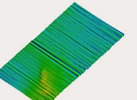
Offshore Argentina Multi beam processed survey
data with latency issues.
As
opposed to all other corrections, the latency value is subtracted from the time tags. This is one of the rare cases where we write
“corrected” values in raw data files.
Offshore Argentina Multi beam processed survey data
with resolved latency issues.
Even
after correcting data for latency we need time synchronization as there are errors affecting the calculated latency value:
• Not running the two lines
exactly one on top of the other
• Changes in depth
correction factors (tide, draft, sound velocity)
• Jumps in position due to
poor GPS positioning or reflections (bridges, piers, vessels, etc.)
• GPS position quality,
offsets, survey conditions, offline distance and even computer ports can
influence the latency. (…preferably use Com 1 &do not use USB to serial
adapters!!).
Don’t
base your latency value on one test! Run as many lines as possible and take an average.
Run your lines as close to the planned line as you can and scrutinize those graphs
and profiles!
Also,
the latency value can change depending on factors such as the number of
satellites.
Therefore we try to synchronize the
computer clock with the GPS clock and take advantage of the time of
applicability contained in the GPS messages. If we can synchronize the two
clocks, we can use the time tags provided by the GPS receiver for data coming
from it and the synchronized computer clock for data coming from other devices
like the echo sounder. For this purpose as mentioned earlier NMEA ZDA message
that seems almost perfect for this purpose as it contains just the GPS time and
date.
How
it all evolved:
Years
ago we used a fairly naive approach to synchronization where we would take the ZDA
message and set the computer clock to the time indicated in that message. The
problem with this approach is that the two clocks can (and will) drift in time
and, unfortunately, you cannot redo the synchronization in the middle of
logging a data file because it would wreak havoc with all the time tags.
This
is a software loop (In electronics terms call it a PLL {Phase Lock Loop}) that
constantly monitors the difference between the GPS clock and the computer clock
and slowly changes the computer clock to match the GPS clock. This basically
was a time management model. If you turn on synchronization and you run the
latency test you should obtain latency very close to 0.
The
latency is not always Zero when using synchronization. Sometimes the resulting latency is still
quite appreciable and this has to do with how the ZDA message is sent.
In the NMEA standard there is no, specification that the
ZDA message should be exactly on the integer second or about the accuracy of
the time indicated in the message. If we look at a typical ZDA message:
$GPZDA,163448.014,09,03,2011,00,00*57
We see that the GPS unit bothered to output the time to
milliseconds resolution so we can hope that it started to send the ZDA message
at that exact moment. This is however not the norm for all GPS receivers. Other
receivers could send the same message as:
$GPZDA,163448,09,03,2011,00,00
(Without any milliseconds) and
send it somewhere during that second but without paying much attention to its
timing.
If
the GPS sends ZDA messages more often than once per second there is a complete
mayhem! Veritime will jump off its rails and very soon you will see the dreaded
“SYNC FAIL” error in the Pulse synchronization program. For fans of
electronics, each PLL loop has a certain bandwidth and sending ZDA messages
more often than once per second falls outside the Veritime bandwidth.
In
case the ZDA messages are sent less than one per second (once every 2 or 5
seconds). It will work, without doing any good, because the time management model will adjust
the clock model only when it receives a ZDA message, we are allowing the two
clocks to drift apart for a longer interval.
The pulse per second output
from the GPS receiver. This is an electrical pulse that we bring through a
small level converter to a RS-232 pin (the CTS signal) and use it as reference
to our PLL loop instead of the ZDA message. To use
the PPS pulse we need a “PPS box” that does the electrical adaptation of the GPS
signal to the RS-232 levels.
The ZDA message is still needed because we need to know the
clock reading when the PPS pulse occurred. This is the most accurate method one
can currently use to synchronize the GPS and computer clock.
As a rule of thumb: the latency errors we can expect are:
• Latency test software: 50 to 100ms
but can change unexpectedly.
• ZDA message for time sync: 20-30 ms;
good enough for singlebeam.
• PPS signal for time sync: 1-5 ms;
good for multibeam.
To check synchronization or compare
the PPS pulse to the ZDA message, the “ZDA time plot” program that
shows a graph of the synchronization error between the GPS clock and the
computer clock.
In
case the synchronization doesn’t work on the computer, take heart in knowing that you aren’t the only one, it’s the possibly the
hardware.
Suggested
workarounds:
Windows XP systems.
Open the
System properties dialog box (Control Panel -> System) and select the “Advanced” tab and under ‘Start up and Recovery’, click [Settings].

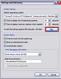
Add the string “/useptimer” at the end
of the line with the operating system.
Save the
file and reboot your system.

Windows 7
Disable “Intel SpeedSetp Technology” in
your BIOS settings.
Go ahead investigating and do keep me posted...
In Multibeam systems, where these echosounders are also fed
the PPS pulse from the GPS, it sends UTC time-tagged data output, QINSy time
tags the other system inputs. Similar options for time tagging are available in
the POS/MV.
We are
coming to a phase where all systems will be time tagging their data and be
getting synchronized; thereby latency concerns will be reduced (if not removed).
So we are good!!! Gracious amigos!